In previous blog posts I presented an introduction to R in eight steps:
step 1: Installation of R and RStudio.
step 2: Set working directory and load data.
step 3: Variables and data types.
step 4: Vector slices and linear regression.
step 5: Vector arithmetic and data frames.
step 6: for loops
step 7: Define a procedure and use if ... else.
step 8: Install packages and use external libraries.
I called it "My introduction ..." because it emphasizes what I find important and interesting in R, rather than a tutorial of R as just another programming language.
Perhaps R is an acquired taste, but it has become one of my preferred tools to understand the world ...
My introduction to R - step 8
R is open source and many people have contributed and continue to contribute procedures, libraries and packages - and we have access to all of them.
Perhaps we want to take a look at kernel regression, one of many machine learning methods.
Wikipedia even has a script for us.
In order to try out the procedure npreg(), we install the package np and open its library of procedures
install.packages("np")
library("np")
Instead of using the procedure install.packages() one can also select Tools > Install Packages ... from the RStudio menu.
We then load the data we want to examine
ryder = read.csv("R.csv",header=T)
In this example, we try to explain the volume (in thousand shares) from the high - low range
y = 0.0001*ryder$Volume
x = ryder$High - ryder$Low
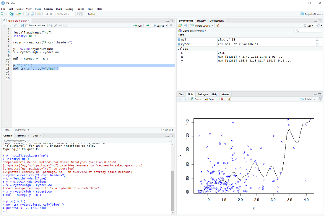
Now we can build the non-parmateric model
mdl = npreg( y ~ x )
and display it together with the data points
plot( mdl )
points( x, y, col="blue" )
exercise: Put the cursor next to the npreg procedure and hit F1 to get the help file. This tells us that npreg uses the parameter bws to set the bandwith (we just used a default). Use the procedure npregbw() to calculate the bandwith before calling npreg.
Hint: There are examples at the end of the helpfile ...
Perhaps we want to take a look at kernel regression, one of many machine learning methods.
Wikipedia even has a script for us.
In order to try out the procedure npreg(), we install the package np and open its library of procedures
install.packages("np")
library("np")
Instead of using the procedure install.packages() one can also select Tools > Install Packages ... from the RStudio menu.
We then load the data we want to examine
ryder = read.csv("R.csv",header=T)
In this example, we try to explain the volume (in thousand shares) from the high - low range
y = 0.0001*ryder$Volume
x = ryder$High - ryder$Low
Now we can build the non-parmateric model
mdl = npreg( y ~ x )
and display it together with the data points
plot( mdl )
points( x, y, col="blue" )
exercise: Put the cursor next to the npreg procedure and hit F1 to get the help file. This tells us that npreg uses the parameter bws to set the bandwith (we just used a default). Use the procedure npregbw() to calculate the bandwith before calling npreg.
Hint: There are examples at the end of the helpfile ...
My introduction to R - step 7
We have used several procedures that come with the R base installation, e.g. plot, lm, read.csv, etc.
But we can also define our own procedures.
In the previous step we calculated the "exponential moving average" of a series of prices; perhaps we want to do this more than once.
In this case it makes sense to define a procedure, which we will call MyEma
MyEma = function( prc ){
L = length(prc)
ema = numeric(L)
ema[1] = prc[1]
for( i in 2:L ){
ema[i] = 0.9*ema[i-1] + 0.1*ryder$Close[i]
}
return(ema)
}
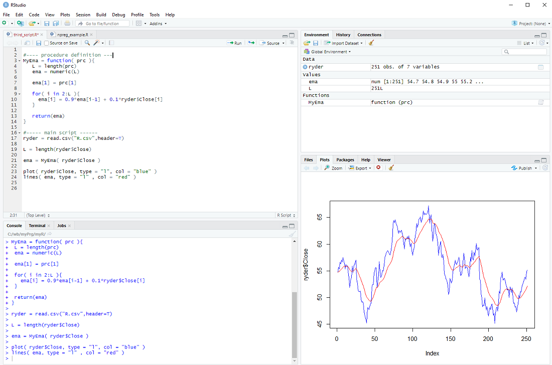
We define our procedure MyEma to have 1 parameter, a vector of prices, then we perform the same calculation as in the previous step (you can actually copy and paste the code) and finally we return the exponential moving average vector as the result of our procedure.
In the main body of our script we can then call the procedure
ema = MyEma( ryder$Close )
with ryder$Close as the input.
If all goes well the plot should be the same as in the previous step ...
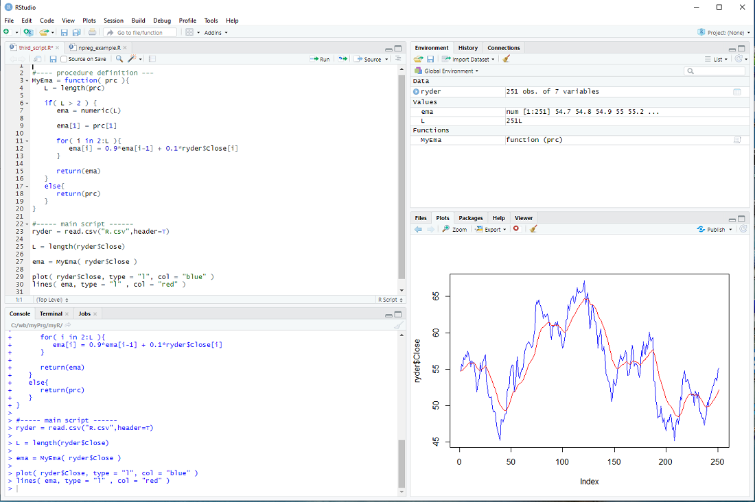
There is only one issue: The loop assumes that there is more than one element in the vector prc and the whole procedure makes little sense if there are less than 3 elements in the prc vector. We should therefore check the length L and only do the loop IF L is larger than 2, otherwise just return the prc as it is.
if( L > 2 ){
for-loop
} else{
return(prc)
}
This is depicted below.
exercise: Use a 2nd parameter w in MyEma, so that
MyEma = function( prc, w ){
and
ema[i] = (1.0 - w)*ema[i-1] + w*ryder$Close[i]
Call MyEma with different values of w and check how the plot changes
MyEma( ryder$Close, 0.1)
MyEma( ryder$Close, 0.05)
MyEma( ryder$Close, 0.2)
etc.
But we can also define our own procedures.
In the previous step we calculated the "exponential moving average" of a series of prices; perhaps we want to do this more than once.
In this case it makes sense to define a procedure, which we will call MyEma
MyEma = function( prc ){
L = length(prc)
ema = numeric(L)
ema[1] = prc[1]
for( i in 2:L ){
ema[i] = 0.9*ema[i-1] + 0.1*ryder$Close[i]
}
return(ema)
}
We define our procedure MyEma to have 1 parameter, a vector of prices, then we perform the same calculation as in the previous step (you can actually copy and paste the code) and finally we return the exponential moving average vector as the result of our procedure.
In the main body of our script we can then call the procedure
ema = MyEma( ryder$Close )
with ryder$Close as the input.
If all goes well the plot should be the same as in the previous step ...
There is only one issue: The loop assumes that there is more than one element in the vector prc and the whole procedure makes little sense if there are less than 3 elements in the prc vector. We should therefore check the length L and only do the loop IF L is larger than 2, otherwise just return the prc as it is.
if( L > 2 ){
for-loop
} else{
return(prc)
}
This is depicted below.
exercise: Use a 2nd parameter w in MyEma, so that
MyEma = function( prc, w ){
and
ema[i] = (1.0 - w)*ema[i-1] + w*ryder$Close[i]
Call MyEma with different values of w and check how the plot changes
MyEma( ryder$Close, 0.1)
MyEma( ryder$Close, 0.05)
MyEma( ryder$Close, 0.2)
etc.
My introduction to R - step 6
Many investors prefer to sell stocks if they "enter into a down trend" - they use e.g. an exponential moving average and sell if the price falls below it.
It is not clear if this actually improves the performance of a a stock portfolio, but perhaps investors sleep better using this approach ...
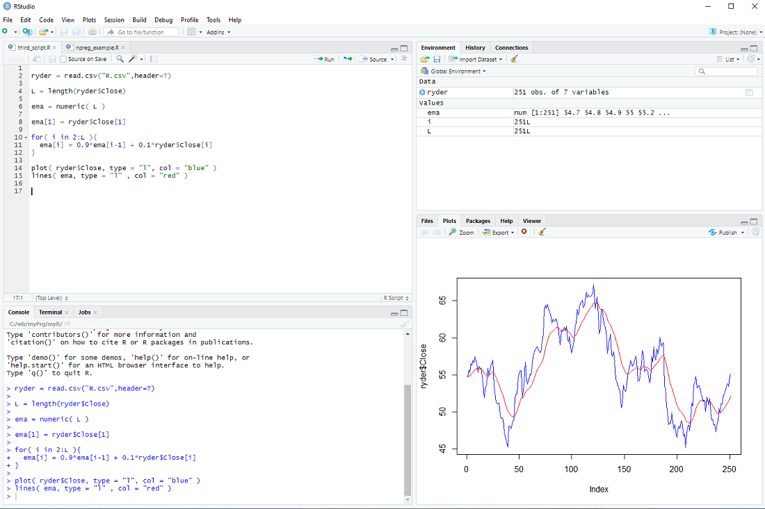
There is no "exponential moving average" procedure in the R base package, but it can be easily calculated with a for-loop.
After loading the stock data file
ryder = read.csv("R.csv",header=T)
L = length(ryder$Close)
we create the vector ema
ema = numeric( L )
We set the first element of ema to the first close price
ema[1] = ryder$Close[1]
and then we calculate
ema[2] = 0.9*ema[1] + 0.1*ryder$[2]
ema[3] = 0.9*ema[2] + 0.1*ryder$[3]
.
.
.
in a loop:
for( i in 2:L ){
ema[i] = 0.9*ema[i-1] + 0.1*ryder$Close[i]
}
Finally, we display the prices and ema
plot( ryder$Close, type = "l", col = "blue" )
lines( ema, type = "l" , col = "red" )
At this point most tutorials would emphasize that R is an interpreted language and for-loops should be avoided at all costs.
Indeed one should use vector operations whenever possible instead of the element-by-element processing in a for loop.
However, microprocessors are so fast nowadays, that for-loops are problematic only for really large data sets imho.
exercise: Repeat the calculation, but with the volume instead of the price.
It is not clear if this actually improves the performance of a a stock portfolio, but perhaps investors sleep better using this approach ...
There is no "exponential moving average" procedure in the R base package, but it can be easily calculated with a for-loop.
After loading the stock data file
ryder = read.csv("R.csv",header=T)
L = length(ryder$Close)
we create the vector ema
ema = numeric( L )
We set the first element of ema to the first close price
ema[1] = ryder$Close[1]
and then we calculate
ema[2] = 0.9*ema[1] + 0.1*ryder$[2]
ema[3] = 0.9*ema[2] + 0.1*ryder$[3]
.
.
.
in a loop:
for( i in 2:L ){
ema[i] = 0.9*ema[i-1] + 0.1*ryder$Close[i]
}
Finally, we display the prices and ema
plot( ryder$Close, type = "l", col = "blue" )
lines( ema, type = "l" , col = "red" )
At this point most tutorials would emphasize that R is an interpreted language and for-loops should be avoided at all costs.
Indeed one should use vector operations whenever possible instead of the element-by-element processing in a for loop.
However, microprocessors are so fast nowadays, that for-loops are problematic only for really large data sets imho.
exercise: Repeat the calculation, but with the volume instead of the price.
My introduction to R - step 5
An important feature of R is that one calculates with vectors and therefore can process large quantities of data in a single line.
Let's take the data from previous steps
ryder = read.csv("R.csv",header=T)
and calculate the "trading range", normalized by the open, for every day
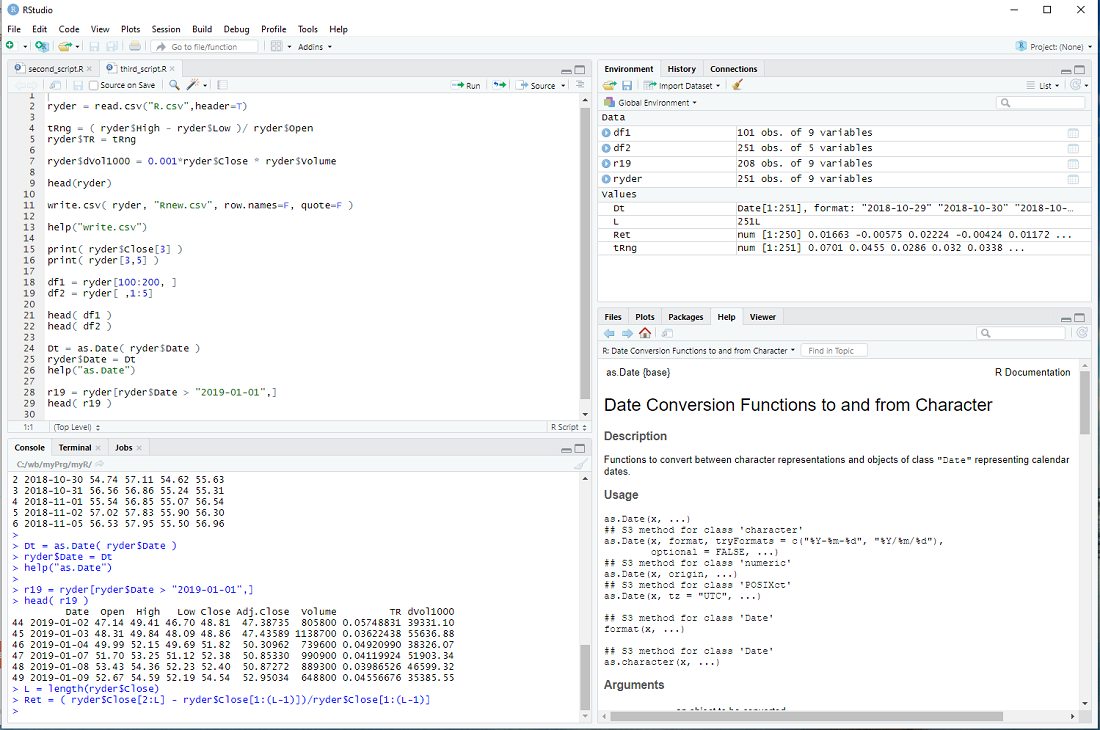
tRng = ( ryder$High - ryder$Low )/ ryder$Open
This generates the vector tRng , calculates the difference of high and low for every day, divided by the open and assigns the result to the elements of tRng, i.e. 251 * 2 calculations, all in one line.
We can now add this vector to the data frame ryder
ryder$TR = tRng
Now let's calculate the dollar trading volume in thousands for each day and add it as a column
ryder$dVol1000 = 0.001*ryder$Close * ryder$Volume
We can take a look at the first entries of the data frame with the head() procedure
head(ryder)
but we would see the same thing in window 3 top right.
If we want to store the expanded data frame in a file, we could do it as follows
write.csv( ryder, "Rnew.csv", row.names=F, quote=F )
I set the parameters so that it has the exact same format as R.csv.
You can get help with
help("write.csv")
The columns of ryder are: Date, Open, High, Low, Close, Adj.Close, Volume, ...
and we can access each column by its name
print( ryder$Close[3] )
But we can also access the elements of a data frame directly
print( ryder[3,5] )
The first index is the row and the second the column (Close is the 5-th column of ryder).
We can also slice data frames
df1 = ryder[100:200, ]
head( df1 )
Notice that the blank entry, instead of an index, means all columns.
df2 = ryder[ , 1:5]
head( df2 )
The blank entry, instead of an index, means all rows.
Until now, I have not mentioned the column Date and for a good reason - it is a bit of a mess.
The read.csv procedure interprets it as a Factor and not a date, although the entries are formatted so that R can interpret it as date.
But we can fix that
Dt = as.Date( ryder$Date )
ryder$Date = Dt
help("as.Date")
The as. family of conversion functions is quite useful in R.
This allows us to slice the data frame ryder in yet another way ...
r19 = ryder[ryder$Date > "2019-01-01",]
head( r19 )
... and concludes this step of my introduction.
exercise: Calculate the returns of ryder for each day, beginning with the 2nd day.
The return on the 2nd day is ( ryder$Close[2] - ryder$Close[1] )/ryder$Close[1] ,
the return on the 3rd day is ( ryder$Close[3] - ryder$Close[2] )/ryder$Close[2] ,
etc. Now calculate it in one line and assign the results to a vector Ret.
hint: Use L = length(ryder$Close) in your calculation ...
Let's take the data from previous steps
ryder = read.csv("R.csv",header=T)
and calculate the "trading range", normalized by the open, for every day
tRng = ( ryder$High - ryder$Low )/ ryder$Open
This generates the vector tRng , calculates the difference of high and low for every day, divided by the open and assigns the result to the elements of tRng, i.e. 251 * 2 calculations, all in one line.
We can now add this vector to the data frame ryder
ryder$TR = tRng
Now let's calculate the dollar trading volume in thousands for each day and add it as a column
ryder$dVol1000 = 0.001*ryder$Close * ryder$Volume
We can take a look at the first entries of the data frame with the head() procedure
head(ryder)
but we would see the same thing in window 3 top right.
If we want to store the expanded data frame in a file, we could do it as follows
write.csv( ryder, "Rnew.csv", row.names=F, quote=F )
I set the parameters so that it has the exact same format as R.csv.
You can get help with
help("write.csv")
The columns of ryder are: Date, Open, High, Low, Close, Adj.Close, Volume, ...
and we can access each column by its name
print( ryder$Close[3] )
But we can also access the elements of a data frame directly
print( ryder[3,5] )
The first index is the row and the second the column (Close is the 5-th column of ryder).
We can also slice data frames
df1 = ryder[100:200, ]
head( df1 )
Notice that the blank entry, instead of an index, means all columns.
df2 = ryder[ , 1:5]
head( df2 )
The blank entry, instead of an index, means all rows.
Until now, I have not mentioned the column Date and for a good reason - it is a bit of a mess.
The read.csv procedure interprets it as a Factor and not a date, although the entries are formatted so that R can interpret it as date.
But we can fix that
Dt = as.Date( ryder$Date )
ryder$Date = Dt
help("as.Date")
The as. family of conversion functions is quite useful in R.
This allows us to slice the data frame ryder in yet another way ...
r19 = ryder[ryder$Date > "2019-01-01",]
head( r19 )
... and concludes this step of my introduction.
exercise: Calculate the returns of ryder for each day, beginning with the 2nd day.
The return on the 2nd day is ( ryder$Close[2] - ryder$Close[1] )/ryder$Close[1] ,
the return on the 3rd day is ( ryder$Close[3] - ryder$Close[2] )/ryder$Close[2] ,
etc. Now calculate it in one line and assign the results to a vector Ret.
hint: Use L = length(ryder$Close) in your calculation ...
My introduction to R - step 4
Linear regression is the oldest machine learning method. It is widely used and allows one to extrapolate from the known to the unknown.
Large fortunes have been made and lost with the help of linear regression models ...
In the following we will calculate a linear model on a sample of stock prices and then compare it against stock prices "out of sample".
If you start RStudio, it might show an R script with leftovers from the previous exercise - I suggest you create a new script (menu bar: File > New File > R Script).
We read the R.csv file from step 2 with read.csv:
ryder = read.csv("R.csv",header=T)
and then store the length of the vector ryder$Close:
L = length(ryder$Close).
We calculate two variables we will later use for displays:
maxP = max(ryder$Close) + 5.0
minP = min(ryder$Close) - 5.0
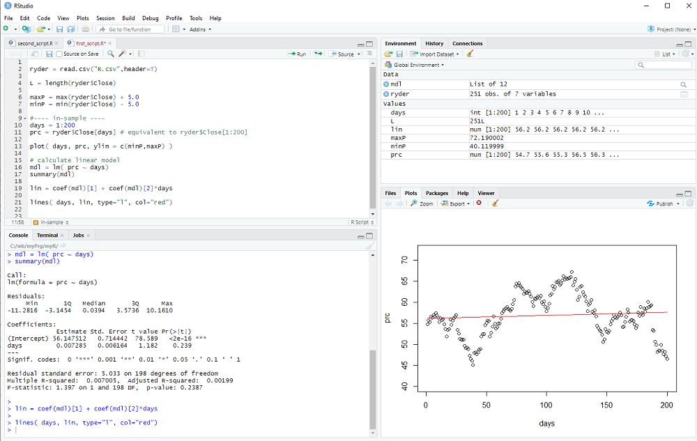
The file should contain more than 250 data points (one year of stock prices) and we use the first 200 days for in sample estimation.
days = 1:200
prc = ryder$Close[days]
Notice that ryder$Close is a vector and ryder$Close[1] is the first element we want and ryder$Close[200] the last of the in-sample period. ryder$Close[days] is equivalent to ryder$Close[1:200] and therefore prc is a vector which stores the first 200 elements of ryder$Close.
This slicing of vectors is quite often used and would work even if the elements of days would not be sequentially ordered.
Now we can plot the prices as a function of each day:
plot( days, prc, ylim = c(minP,maxP) )
We calculate the linear regression model with the lm() procedure:
mdl = lm( prc ~ days)
Notice the ~ used in the procedure call (which may or may not not be easy to find on a non-US keyboard).
We can print a summary of the linear model with
summary(mdl)
and we get the two coefficients (intercept and slope) using coef(mdl), which returns a vector.
Therefore we can calculate the linear model as
lin = coef(mdl)[1] + coef(mdl)[2]*days
and add the line to our plot with the lines() procedure:
lines( days, lin, type="l", col="red")
You can either execute your script step by step with Ctrl-Enter or type the script first and then execute the whole thing by selecting from the menu: Code > Run Region > Run All
Now we look at the out-of-sample data:
days = 201:L
prc = ryder$Close[days]
and display it with
plot( days, prc, ylim = c(minP,maxP) )
We calculate the out-of-sample model
lin = coef(mdl)[1] + coef(mdl)[2]*days
and add the line to the plot
lines( days, lin, type="l", col="red")
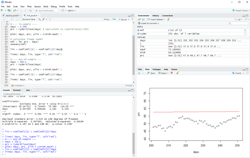
We could now calculate the out-of-sample error (it is quite obvious that the error exceeds the variance of the data in this example 8-) and perhaps repeat the procedure for many different stocks and time periods to check if the linear model has any useful predictive value.
However, this concludes step 4 of my introduction
exercise: Repeat this regression exercise, but use the Volume instead of the Close ...
Large fortunes have been made and lost with the help of linear regression models ...
In the following we will calculate a linear model on a sample of stock prices and then compare it against stock prices "out of sample".
If you start RStudio, it might show an R script with leftovers from the previous exercise - I suggest you create a new script (menu bar: File > New File > R Script).
We read the R.csv file from step 2 with read.csv:
ryder = read.csv("R.csv",header=T)
and then store the length of the vector ryder$Close:
L = length(ryder$Close).
We calculate two variables we will later use for displays:
maxP = max(ryder$Close) + 5.0
minP = min(ryder$Close) - 5.0
The file should contain more than 250 data points (one year of stock prices) and we use the first 200 days for in sample estimation.
days = 1:200
prc = ryder$Close[days]
Notice that ryder$Close is a vector and ryder$Close[1] is the first element we want and ryder$Close[200] the last of the in-sample period. ryder$Close[days] is equivalent to ryder$Close[1:200] and therefore prc is a vector which stores the first 200 elements of ryder$Close.
This slicing of vectors is quite often used and would work even if the elements of days would not be sequentially ordered.
Now we can plot the prices as a function of each day:
plot( days, prc, ylim = c(minP,maxP) )
We calculate the linear regression model with the lm() procedure:
mdl = lm( prc ~ days)
Notice the ~ used in the procedure call (which may or may not not be easy to find on a non-US keyboard).
We can print a summary of the linear model with
summary(mdl)
and we get the two coefficients (intercept and slope) using coef(mdl), which returns a vector.
Therefore we can calculate the linear model as
lin = coef(mdl)[1] + coef(mdl)[2]*days
and add the line to our plot with the lines() procedure:
lines( days, lin, type="l", col="red")
You can either execute your script step by step with Ctrl-Enter or type the script first and then execute the whole thing by selecting from the menu: Code > Run Region > Run All
Now we look at the out-of-sample data:
days = 201:L
prc = ryder$Close[days]
and display it with
plot( days, prc, ylim = c(minP,maxP) )
We calculate the out-of-sample model
lin = coef(mdl)[1] + coef(mdl)[2]*days
and add the line to the plot
lines( days, lin, type="l", col="red")
We could now calculate the out-of-sample error (it is quite obvious that the error exceeds the variance of the data in this example 8-) and perhaps repeat the procedure for many different stocks and time periods to check if the linear model has any useful predictive value.
However, this concludes step 4 of my introduction
exercise: Repeat this regression exercise, but use the Volume instead of the Close ...
My introduction to R - step 3
In the previous two steps we encountered variables and constants of different types.
Let's take a closer look ...
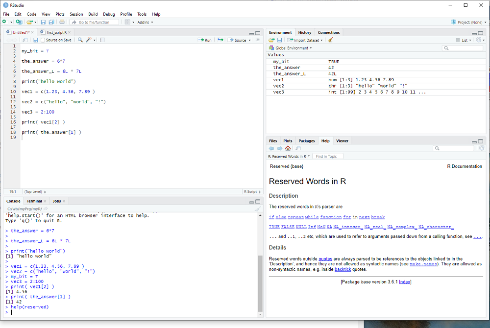
In R one creates variables by giving them a name and assigning a value, as we did with
the_answer = 6*7
The name can consist of letters, numbers and the two characters _ and .
but do not use _ or . or a number as the first character.
Examples of valid names:
var1
the_strength_of_Luisa
dog.leg
There are reserved words, which cannot be used to name variables, you can get a list with the help procedure:
help(reserved)
You probably don't want this line in your R script, so I suggest you type help(reserved) in window 2 bottom left and hit Enter. Indeed window 2 is a fully functional R terminal and I use it to try out things and keep whatever code I want saved in window 1, i.e. in my R script.
Whenever we create a variable, R figures out the data type from the assigned value and/or operation(s).
We already encountered several different data types:
logical: TRUE or FALSE , abbreviated as T or F (e.g. the parameter header=T in the read.csv procedure)
numeric: the_answer = 6*7 was our first example, 3.1415 would be another
integer: R does not distinguish 6 from 6.0 , but if one wants to explicitly use a whole number
it needs do be indicated with the letter L, e.g. 6L
the_answer = 6L*7L
is now an integer and not a numeric variable.
strings: We have used the string "blue" in the plot procedure and one can display strings e.g. with the print procedure
print("blue")
R uses vectors as basic building blocks, collections of elements with the same data type.
ryder$Close was an example of a vector.
But the_answer was a vector too, just a small vector with 1 element only.
We access the elements of a vector with the [] operator, so that
ryder$Close[3]
would be the 3rd element of the vector, i.e. the 3rd entry of the data column.
And the_answer[1] would be the one and only element of the vector the_answer.
Notice that vector indices begin with 1 and not 0 as in some other programming languages.
One can generate a vector e.g. with the function c(), used so often that it has a really short name:
vec1 = c(1.1, 2.7, 3.2, 4.6)
creates a numeric vector with 4 elements.
vec2 = c("me","my","friend","and","you")
creates a vector with 5 strings as elements.
Last but not least, the : operator can be used to create a specific vector of integers
vec3 = 2:7
creates a vector with 5 integers as elements, the whole numbers 2, 3, 4, 5, 6, 7.
exercise: Create vectors of different sizes and types - watch in window 3 what it displays for each one.
Let's take a closer look ...
In R one creates variables by giving them a name and assigning a value, as we did with
the_answer = 6*7
The name can consist of letters, numbers and the two characters _ and .
but do not use _ or . or a number as the first character.
Examples of valid names:
var1
the_strength_of_Luisa
dog.leg
There are reserved words, which cannot be used to name variables, you can get a list with the help procedure:
help(reserved)
You probably don't want this line in your R script, so I suggest you type help(reserved) in window 2 bottom left and hit Enter. Indeed window 2 is a fully functional R terminal and I use it to try out things and keep whatever code I want saved in window 1, i.e. in my R script.
Whenever we create a variable, R figures out the data type from the assigned value and/or operation(s).
We already encountered several different data types:
logical: TRUE or FALSE , abbreviated as T or F (e.g. the parameter header=T in the read.csv procedure)
numeric: the_answer = 6*7 was our first example, 3.1415 would be another
integer: R does not distinguish 6 from 6.0 , but if one wants to explicitly use a whole number
it needs do be indicated with the letter L, e.g. 6L
the_answer = 6L*7L
is now an integer and not a numeric variable.
strings: We have used the string "blue" in the plot procedure and one can display strings e.g. with the print procedure
print("blue")
R uses vectors as basic building blocks, collections of elements with the same data type.
ryder$Close was an example of a vector.
But the_answer was a vector too, just a small vector with 1 element only.
We access the elements of a vector with the [] operator, so that
ryder$Close[3]
would be the 3rd element of the vector, i.e. the 3rd entry of the data column.
And the_answer[1] would be the one and only element of the vector the_answer.
Notice that vector indices begin with 1 and not 0 as in some other programming languages.
One can generate a vector e.g. with the function c(), used so often that it has a really short name:
vec1 = c(1.1, 2.7, 3.2, 4.6)
creates a numeric vector with 4 elements.
vec2 = c("me","my","friend","and","you")
creates a vector with 5 strings as elements.
Last but not least, the : operator can be used to create a specific vector of integers
vec3 = 2:7
creates a vector with 5 integers as elements, the whole numbers 2, 3, 4, 5, 6, 7.
exercise: Create vectors of different sizes and types - watch in window 3 what it displays for each one.
My introduction to R - step 2
R is mainly used for statistics, machine learning etc. and to do that we need interesting data.
One place which generates a lot of data is the US stock market and therefore we head over to
finance.yahoo.com
to grab some interesting free samples.
On the right hand side there is a box Quote Lookup and we enter R as the ticker symbol, which gives us price and other information for Ryder System Inc. - a company which has little to do with the R programming language.
We click on historical data, select a time period (1 year is fine), push the "Apply" button and then click on "Download Data".
Save the file R.csv to the myR folder (or wherever you like to store it).
Now it is time to start RStudio and it will probably open with the one-line script we made in the previous step.
However, we already know the_answer and we "comment out the line" by putting a # character in front of it.
R ignores comments and RStudio colors them green, they are only there for us human beings to better understand what we did and want to do ...
Before we take a look at the R.csv file, we set the "working directory" in RStudio: In the menu click on Tools and select Tools > Global Options ... and then select General (which should be the default selection anyways). Go to "Default working directory ..." and select the path to your myR folder (or wherever you stored the R.csv file) by pushing the Browse button; then hit apply and eventually this will need a restart of RStudio to take effect.
Alternatively, one can call the R procedure setwd in the R script to set that path:
setwd("c:/path/to/my/folder/myR")
Notice that R uses forward slashes, even on windows, betraying its unix heritage.
Now we are ready to load the stock data of Ryder System Inc. using the read.csv procedure:
ryder = read.csv( "R.csv", header=T )
After we execute the line with Ctrl-Enter, window 3 top right will display the variable ryder and by clicking on the arrow next to it we see more of what it contains.
This is how RStudion looks at this point:
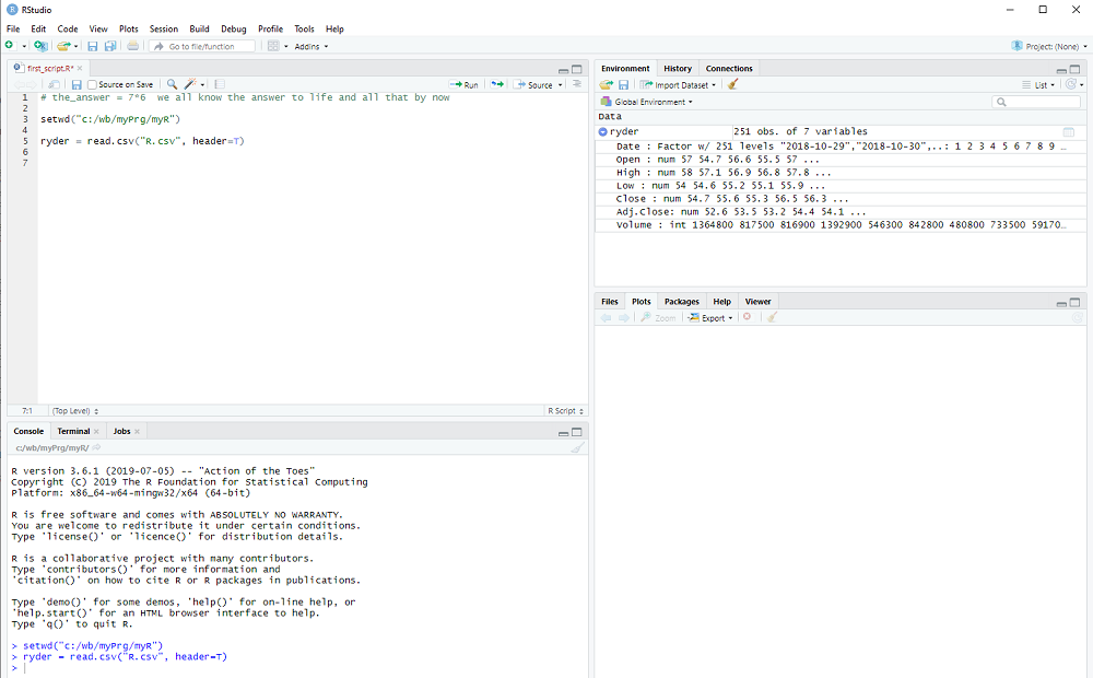
The columns that we saw on the Yahoo webpage are all there: Date, Open, High, ...
R tells us what type they are, num for decimal number, int for integers, etc. and shows us some examples.
In other words, read.csv converts the comma separated values (aha, this is what csv stands for) of the file into a collection of variables, which is called dataframe in R.
We can access each column in the dataframe using its name and the $ operator, e.g. ryder$Close
This works, because we used header=T in the read.csv procedure (T stands for TRUE).
If the data comes in a different file format, e.g. variables separated by tabs is popular, the read.table procedure might be used to import data into R.
We will now take a first look at the data using the plot procedure:
plot( ryder$Close, type="l", col="blue" )
You may notice that a window popped up, listing the available columns in ryder while you typed. You can use that window to select Close without further typing.
RStudio now looks like this:
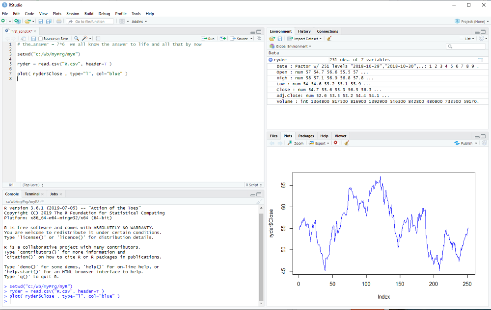
This concludes the 2nd step of my introduction. Don't forget to save your R script with File > Save in the menubar.
exercise: Click on the line with the plot procedure and then hit F1. The help text for the plot procedure should appear in window 4, bottom right.
Try different types and colors with your plot ...
One place which generates a lot of data is the US stock market and therefore we head over to
finance.yahoo.com
to grab some interesting free samples.
On the right hand side there is a box Quote Lookup and we enter R as the ticker symbol, which gives us price and other information for Ryder System Inc. - a company which has little to do with the R programming language.
We click on historical data, select a time period (1 year is fine), push the "Apply" button and then click on "Download Data".
Save the file R.csv to the myR folder (or wherever you like to store it).
Now it is time to start RStudio and it will probably open with the one-line script we made in the previous step.
However, we already know the_answer and we "comment out the line" by putting a # character in front of it.
R ignores comments and RStudio colors them green, they are only there for us human beings to better understand what we did and want to do ...
Before we take a look at the R.csv file, we set the "working directory" in RStudio: In the menu click on Tools and select Tools > Global Options ... and then select General (which should be the default selection anyways). Go to "Default working directory ..." and select the path to your myR folder (or wherever you stored the R.csv file) by pushing the Browse button; then hit apply and eventually this will need a restart of RStudio to take effect.
Alternatively, one can call the R procedure setwd in the R script to set that path:
setwd("c:/path/to/my/folder/myR")
Notice that R uses forward slashes, even on windows, betraying its unix heritage.
Now we are ready to load the stock data of Ryder System Inc. using the read.csv procedure:
ryder = read.csv( "R.csv", header=T )
After we execute the line with Ctrl-Enter, window 3 top right will display the variable ryder and by clicking on the arrow next to it we see more of what it contains.
This is how RStudion looks at this point:
The columns that we saw on the Yahoo webpage are all there: Date, Open, High, ...
R tells us what type they are, num for decimal number, int for integers, etc. and shows us some examples.
In other words, read.csv converts the comma separated values (aha, this is what csv stands for) of the file into a collection of variables, which is called dataframe in R.
We can access each column in the dataframe using its name and the $ operator, e.g. ryder$Close
This works, because we used header=T in the read.csv procedure (T stands for TRUE).
If the data comes in a different file format, e.g. variables separated by tabs is popular, the read.table procedure might be used to import data into R.
We will now take a first look at the data using the plot procedure:
plot( ryder$Close, type="l", col="blue" )
You may notice that a window popped up, listing the available columns in ryder while you typed. You can use that window to select Close without further typing.
RStudio now looks like this:
This concludes the 2nd step of my introduction. Don't forget to save your R script with File > Save in the menubar.
exercise: Click on the line with the plot procedure and then hit F1. The help text for the plot procedure should appear in window 4, bottom right.
Try different types and colors with your plot ...
My introduction to R - step 1
You want to know how to actually do machine learning, or you want to know how those finance quants do their job, or you just want
to add a valuable skill to your cv ...
In other words, you want to learn R (btw what programming language do pirates use? Rrrrrrr ).
But you want to learn in small steps, easy to follow along and yet with visible results already after a few steps. Well, you have come to the right place and as additional benefit you can post questions and comments whenever you want or need to know more ...
Just one important disclaimer: I am just another user, perhaps with a bit more experience than you at the moment; but I still peek into my R for Dummies book every now and then.
I am certainly not an R guru.
The first thing we need to do is install R and Rstudio.
Install R: Go to www.r_project.org, click on download R and select a mirror.
If you live e.g. in the UK, you might select the one from Imperial College of London.
There you select your operating system and click on install R for the first time (if you are on Windows) or save the R-3.61.pkg package (if you are on a Mac), or whatever is the latest package. Linux users need to select their distribution etc.
Install RStudio: Go to rstudio.com and click on the download rstudio button. Choose the free version of RStudio Desktop and select the installer for your operating system or Linux distribution etc. ...
If you have problems with the installation, please post a comment or ask Google for help.
But if all goes well, you should be able to start RStudio and it will look like this:
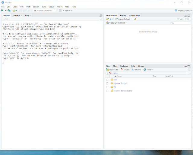
Click on File in the menu bar and select File > New File > R script.
RStudio will now look like this:
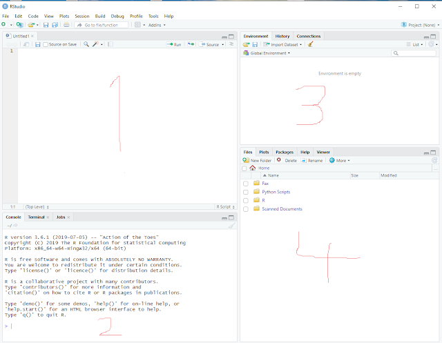
It contains 4 sub-windows and I have scribbled numbers into the screenshot to better explain what they are.
1> top left: This window displays our R script and we will edit it there.
2> bottom left: This window shows executed commands, error messages, etc.
3> top right: This window shows all the different data and variables we will generate.
4> bottom right: This window is used for various displays, help text etc.
In order to get really started, we type our first R script in sub-window 1 and it contains only one line:
the_answer = 7*6
After typing that, with the cursor still on the line, press Ctrl-Enter to "execute" it.
Alternatively, we could have selected Code from the menu bar and then "Run Selected Line(s)".
The RStudio screen should now look like this:
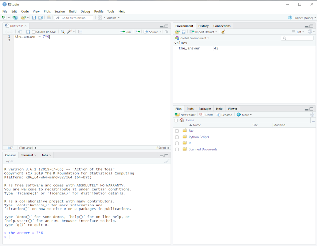
In the top left window 1 we still see our R script, containing one line.
In the bottom left window 2 we see that R executed our line without error and
in the top right window 3 we see that R created a variable named the_answer with the value 42.
R actually did three things: It created the_answer, executed the arithmetic operation 7*6 and then assigned the outcome of that operation to the_answer.
I read that some people have a problem with the = operator when learning to program in some cases. R has a solution for that, one can also use the assignment operator <- instead of the equal sign. So we could have written
the_answer <- 7*6
with the exact same outcome. In older texts this assignment operator is often used instead of = and you should know that it really makes no difference.
Now we want to save our script and I recommend that you create a folder somewhere on your pc, which you will use to store the R scripts and data files we use in this tutorial; I named my folder myR and will reference it in future steps with this name.
Once you have created and/or selected a place on your pc, select File on the menu bar, click on Save As..., navigate to myR and choose a name for your script, e.g. first_step.R
I recommend that your script files end with .R
This concludes the first step of my introduction.
exercise: Click on Help in the menu bar, select R Help and browse e.g. "An Introduction to R", in window 4.
Just one more thing. At the end of your RStudio exercise, select File from the menu and click on Quit Session...; if you are prompted to save the workspace image select No, which means that the next time you start RStudio, you start from a clean slate.
In other words, you want to learn R (btw what programming language do pirates use? Rrrrrrr ).
But you want to learn in small steps, easy to follow along and yet with visible results already after a few steps. Well, you have come to the right place and as additional benefit you can post questions and comments whenever you want or need to know more ...
Just one important disclaimer: I am just another user, perhaps with a bit more experience than you at the moment; but I still peek into my R for Dummies book every now and then.
I am certainly not an R guru.
The first thing we need to do is install R and Rstudio.
Install R: Go to www.r_project.org, click on download R and select a mirror.
If you live e.g. in the UK, you might select the one from Imperial College of London.
There you select your operating system and click on install R for the first time (if you are on Windows) or save the R-3.61.pkg package (if you are on a Mac), or whatever is the latest package. Linux users need to select their distribution etc.
Install RStudio: Go to rstudio.com and click on the download rstudio button. Choose the free version of RStudio Desktop and select the installer for your operating system or Linux distribution etc. ...
If you have problems with the installation, please post a comment or ask Google for help.
But if all goes well, you should be able to start RStudio and it will look like this:
Click on File in the menu bar and select File > New File > R script.
RStudio will now look like this:
It contains 4 sub-windows and I have scribbled numbers into the screenshot to better explain what they are.
1> top left: This window displays our R script and we will edit it there.
2> bottom left: This window shows executed commands, error messages, etc.
3> top right: This window shows all the different data and variables we will generate.
4> bottom right: This window is used for various displays, help text etc.
In order to get really started, we type our first R script in sub-window 1 and it contains only one line:
the_answer = 7*6
After typing that, with the cursor still on the line, press Ctrl-Enter to "execute" it.
Alternatively, we could have selected Code from the menu bar and then "Run Selected Line(s)".
The RStudio screen should now look like this:
In the top left window 1 we still see our R script, containing one line.
In the bottom left window 2 we see that R executed our line without error and
in the top right window 3 we see that R created a variable named the_answer with the value 42.
R actually did three things: It created the_answer, executed the arithmetic operation 7*6 and then assigned the outcome of that operation to the_answer.
I read that some people have a problem with the = operator when learning to program in some cases. R has a solution for that, one can also use the assignment operator <- instead of the equal sign. So we could have written
the_answer <- 7*6
with the exact same outcome. In older texts this assignment operator is often used instead of = and you should know that it really makes no difference.
Now we want to save our script and I recommend that you create a folder somewhere on your pc, which you will use to store the R scripts and data files we use in this tutorial; I named my folder myR and will reference it in future steps with this name.
Once you have created and/or selected a place on your pc, select File on the menu bar, click on Save As..., navigate to myR and choose a name for your script, e.g. first_step.R
I recommend that your script files end with .R
This concludes the first step of my introduction.
exercise: Click on Help in the menu bar, select R Help and browse e.g. "An Introduction to R", in window 4.
Just one more thing. At the end of your RStudio exercise, select File from the menu and click on Quit Session...; if you are prompted to save the workspace image select No, which means that the next time you start RStudio, you start from a clean slate.
quora
CIP mentioned quora and I found a few interesting pictures there ...

Nereis Sandersi, a deep sea vent worm.

Red blood cell on a needle.

Human embryo on a pin.
Nereis Sandersi, a deep sea vent worm.
Red blood cell on a needle.
Human embryo on a pin.
Where have all the crackpots gone?
Crazy people are still everywhere, but I am interested in the special case of physics and math crackpots.
In the good old days of webpages, usenet and blogs they were always there, explaining the real truth about physics and math
with their animated gifs and blinking headlines.
I remember quantoken, plato, plutonium and a young lady who was convinced black holes are driving volcanoes, but there were many more and it seems that they all disappeared from my internet.
What happened to the crackpots?
Perhaps my internet habits changed, but google trends suggests that something changed indeed.
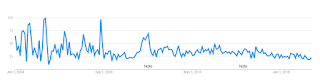
google trends: "crackpot", 2004 - 2019
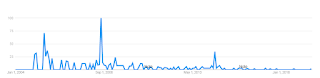
google trends: "crackpot index", 2004 - 2019
I am thinking "crackpot index" is a good proxy for a search related to physics and math crackpots.
Furthermore, I did a simple twitter search for "crackpot" and "crackpot physics" and found nothing related to the category I am talking about.
There is still viXra, but the number of papers posted there is surprisingly small (a total of 31k vs 1.5M on arXiv *).
So what happened to them? Did they all move on from disproving relativity and quantum theory to disproving the moon landings? Did they all become 9/11 truthers etc.? Or does the noise and general madness on facebook and twitter drown them out?
They might be an overlooked species, threatened by extinction, if we don't act soon ...
(*) I do not want to suggest that all papers on viXra are crackpot material, I read somewhere that about 15% get published in journals (whatever that means nowadays), and a significant part of arxiv is garbage.
I remember quantoken, plato, plutonium and a young lady who was convinced black holes are driving volcanoes, but there were many more and it seems that they all disappeared from my internet.
What happened to the crackpots?
Perhaps my internet habits changed, but google trends suggests that something changed indeed.
google trends: "crackpot", 2004 - 2019
google trends: "crackpot index", 2004 - 2019
I am thinking "crackpot index" is a good proxy for a search related to physics and math crackpots.
Furthermore, I did a simple twitter search for "crackpot" and "crackpot physics" and found nothing related to the category I am talking about.
There is still viXra, but the number of papers posted there is surprisingly small (a total of 31k vs 1.5M on arXiv *).
So what happened to them? Did they all move on from disproving relativity and quantum theory to disproving the moon landings? Did they all become 9/11 truthers etc.? Or does the noise and general madness on facebook and twitter drown them out?
They might be an overlooked species, threatened by extinction, if we don't act soon ...
(*) I do not want to suggest that all papers on viXra are crackpot material, I read somewhere that about 15% get published in journals (whatever that means nowadays), and a significant part of arxiv is garbage.
How not to die ...
A few things changed during the last six months.
We moved from The Bahamas to Malta; one advantage is that I don't need to follow the track of hurricane Dorian closely.
We moved to a plant based diet, after reading Dr. Greger's book How Not To Die.
If you are worried about heart attack, stroke, cancer and all that you may want to visit his webpage.
Btw a while ago there was some back and forth with CIP about the paleo-diet; meanwhile I learned that the real paleo diet was mostly plant based with very high amounts of fiber.
I go the gym now every day, do breathing exercises and try to improve my sleep; it is not easy getting old.
Last but not least, I try to exercise my brain to delay the onset of dementia - but I forgot why ...
To blog or not to blog ...
... that is the question.
added later:
Sean published yet another book promoting the many worlds interpretation. I did not read it, only saw a short review.
Obviously, they don't read my blog(s) - otherwise they would know why m.w.i does not work: link 1 and link 2.
So why write blog posts that nobody reads? Well, there is a good chance that Black Mirror has it right (as usual); my experience is just the result of some simulation (btw if you believe the m.w.i. then you have to believe that) and so the blog posts I wrote are for a higher being, who certainly appreciates the wisdom of my thoughts, otherwise why would She keep the simulation alive ...
Sabineblogging
Right now it seems to be a thing to have an opinion about S.H.'s opinions (*).
I don't really care that much about her opinions, but as a follower of internet fashion I read her latest blog post and I found the last sentence interesting:
"The easiest way to see that the problem exists is that they deny it."
So you can either agree with her and support her argument, or you can deny it, which also supports her argument.
I find it interesting that the rhetorical tricks of the dark ages are now entering the scientific discourse ...
(*) Btw the comments made by wolfgang over there are not mine.
added much later: It seem that Sabine is going to sue her most aggressive critic in court.
the ABC conjecture
Three people at a party: Alex is married, we don't know much about Betty and Chris is unmarried.
We notice that Alex is constantly staring at Betty, but Betty is only looking at Chris all the time.
This seems to be yet another case of a married person looking for too long at an unmarried person.
But can we be sure? What is the probability that this ABC conjecture is true?
We notice that Alex is constantly staring at Betty, but Betty is only looking at Chris all the time.
This seems to be yet another case of a married person looking for too long at an unmarried person.
But can we be sure? What is the probability that this ABC conjecture is true?
Just some links ...
... you have probably seen before, in other words too little too late as usual.
Oumuamua is probably not an alien spaceship, but there are many weird and mysterious objects in the universe.
I think AlphaFold is so far the most interesting achievement of 'deep learning' and I assume that computational (bio)chemistry will make big steps in coming years.
The paper of Kelly and Trugenberger examines 'combinatorial quantum gravity' on random graphs. I find it very interesting, because they claim to get a 2nd order phase transition, i.e. a continuum limit, not seen in lattice gravity models so far.
A book review and some thoughts about the value of french fries that I found interesting.
Last but not least, a webpage with lots of good news.
1995
When did everything become so stupid?
Recently I was wondering when it happened, perhaps with the idea that it might help identify the cause. I think I found the answer.
It would be easy to set this date at 2016, but I think it would also be wrong; just think about all that happened before.
Of course, stupidity is nothing new, idiotic politicians are nothing new and mass hysteria and conspiracy theories have always been part of history.
But something changed for the worse in the last one or two decades and it all began in 1995 imho.
It was the year of the OJ trial, when news turned into a weird soap opera for the first time and a strange chain of cause and effect gave us the Kardashians.
Around the same time non-linear video editing became available, which initially made reality tv cheap to produce and finally made it possible for everybody to make video clips.
The drudgereport was also launched in 1995, paving the way for breitbart and infowars.
But most importantly, it was the year of win95, which finally made the internet available to everybody with a pc (*).
The avalanche of stupidity that we experience now was an inevitable consequence of that year ...
(*) The Eternal September began already in 1993 and I admit that there is some uncertainty in the exact timing of the onset of the stupidity avalanche.
added later: One other data point to consider is the reversal of the Flynn effect: It suggests that IQ declined for post-1975 cohorts; this decline would have begun to show up in adults around 1995.
Subscribe to:
Posts (Atom)