In previous blog posts I presented an introduction to R in eight steps:
step 1: Installation of R and RStudio.
step 2: Set working directory and load data.
step 3: Variables and data types.
step 4: Vector slices and linear regression.
step 5: Vector arithmetic and data frames.
step 6: for loops
step 7: Define a procedure and use if ... else.
step 8: Install packages and use external libraries.
I called it "My introduction ..." because it emphasizes what I find important and interesting in R, rather than a tutorial of R as just another programming language.
Perhaps R is an acquired taste, but it has become one of my preferred tools to understand the world ...
My introduction to R - step 8
R is open source and many people have contributed and continue to contribute procedures, libraries and packages - and we have access to all of them.
Perhaps we want to take a look at kernel regression, one of many machine learning methods.
Wikipedia even has a script for us.
In order to try out the procedure npreg(), we install the package np and open its library of procedures
install.packages("np")
library("np")
Instead of using the procedure install.packages() one can also select Tools > Install Packages ... from the RStudio menu.
We then load the data we want to examine
ryder = read.csv("R.csv",header=T)
In this example, we try to explain the volume (in thousand shares) from the high - low range
y = 0.0001*ryder$Volume
x = ryder$High - ryder$Low
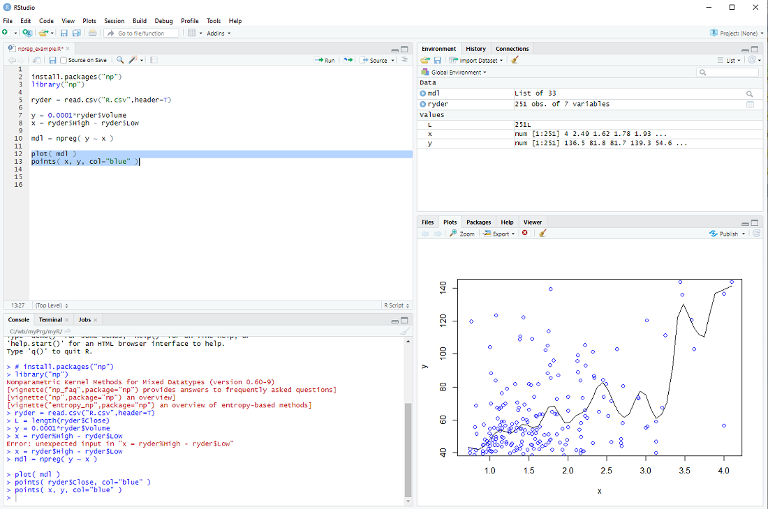
Now we can build the non-parmateric model
mdl = npreg( y ~ x )
and display it together with the data points
plot( mdl )
points( x, y, col="blue" )
exercise: Put the cursor next to the npreg procedure and hit F1 to get the help file. This tells us that npreg uses the parameter bws to set the bandwith (we just used a default). Use the procedure npregbw() to calculate the bandwith before calling npreg.
Hint: There are examples at the end of the helpfile ...
Perhaps we want to take a look at kernel regression, one of many machine learning methods.
Wikipedia even has a script for us.
In order to try out the procedure npreg(), we install the package np and open its library of procedures
install.packages("np")
library("np")
Instead of using the procedure install.packages() one can also select Tools > Install Packages ... from the RStudio menu.
We then load the data we want to examine
ryder = read.csv("R.csv",header=T)
In this example, we try to explain the volume (in thousand shares) from the high - low range
y = 0.0001*ryder$Volume
x = ryder$High - ryder$Low
Now we can build the non-parmateric model
mdl = npreg( y ~ x )
and display it together with the data points
plot( mdl )
points( x, y, col="blue" )
exercise: Put the cursor next to the npreg procedure and hit F1 to get the help file. This tells us that npreg uses the parameter bws to set the bandwith (we just used a default). Use the procedure npregbw() to calculate the bandwith before calling npreg.
Hint: There are examples at the end of the helpfile ...
My introduction to R - step 7
We have used several procedures that come with the R base installation, e.g. plot, lm, read.csv, etc.
But we can also define our own procedures.
In the previous step we calculated the "exponential moving average" of a series of prices; perhaps we want to do this more than once.
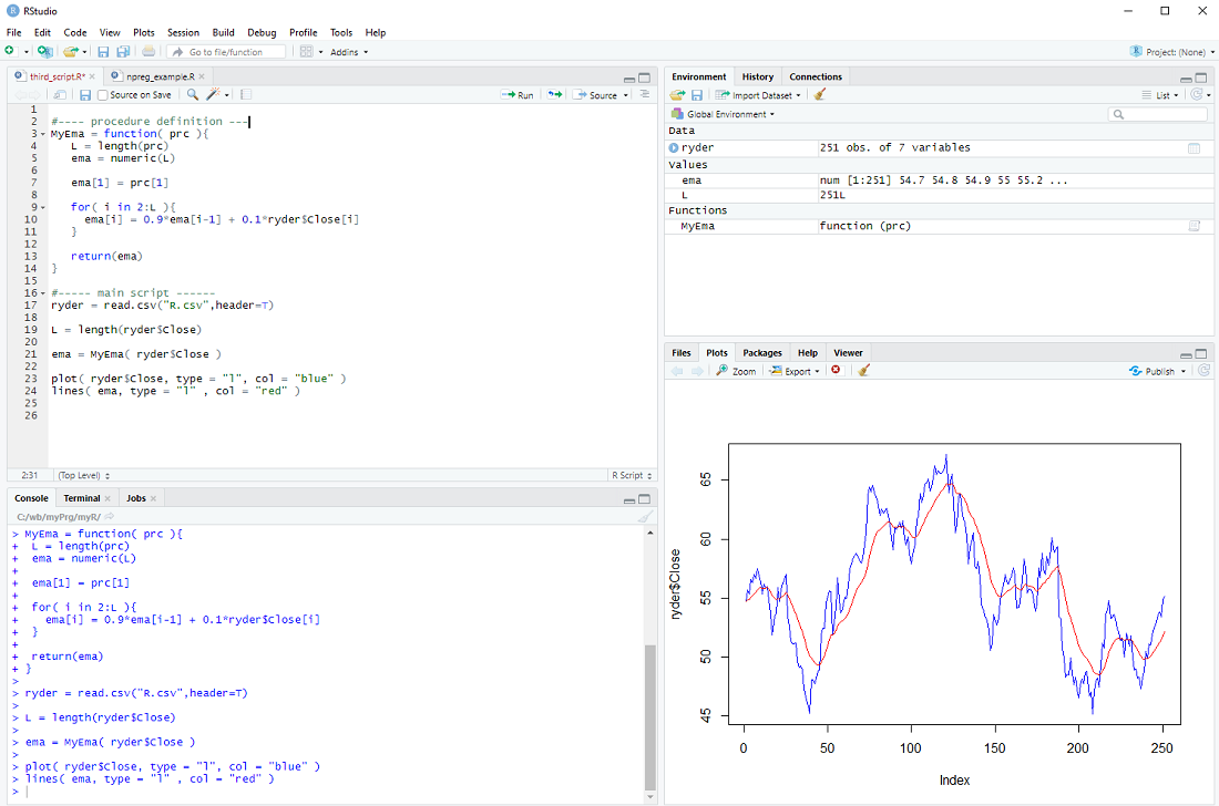
In this case it makes sense to define a procedure, which we will call MyEma
MyEma = function( prc ){
L = length(prc)
ema = numeric(L)
ema[1] = prc[1]
for( i in 2:L ){
ema[i] = 0.9*ema[i-1] + 0.1*ryder$Close[i]
}
return(ema)
}
We define our procedure MyEma to have 1 parameter, a vector of prices, then we perform the same calculation as in the previous step (you can actually copy and paste the code) and finally we return the exponential moving average vector as the result of our procedure.
In the main body of our script we can then call the procedure
ema = MyEma( ryder$Close )
with ryder$Close as the input.
If all goes well the plot should be the same as in the previous step ...
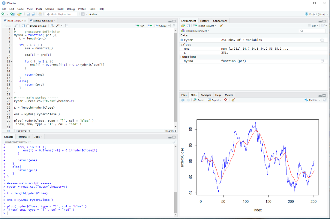
There is only one issue: The loop assumes that there is more than one element in the vector prc and the whole procedure makes little sense if there are less than 3 elements in the prc vector. We should therefore check the length L and only do the loop IF L is larger than 2, otherwise just return the prc as it is.
if( L > 2 ){
for-loop
} else{
return(prc)
}
This is depicted below.
exercise: Use a 2nd parameter w in MyEma, so that
MyEma = function( prc, w ){
and
ema[i] = (1.0 - w)*ema[i-1] + w*ryder$Close[i]
Call MyEma with different values of w and check how the plot changes
MyEma( ryder$Close, 0.1)
MyEma( ryder$Close, 0.05)
MyEma( ryder$Close, 0.2)
etc.
But we can also define our own procedures.
In the previous step we calculated the "exponential moving average" of a series of prices; perhaps we want to do this more than once.
In this case it makes sense to define a procedure, which we will call MyEma
MyEma = function( prc ){
L = length(prc)
ema = numeric(L)
ema[1] = prc[1]
for( i in 2:L ){
ema[i] = 0.9*ema[i-1] + 0.1*ryder$Close[i]
}
return(ema)
}
We define our procedure MyEma to have 1 parameter, a vector of prices, then we perform the same calculation as in the previous step (you can actually copy and paste the code) and finally we return the exponential moving average vector as the result of our procedure.
In the main body of our script we can then call the procedure
ema = MyEma( ryder$Close )
with ryder$Close as the input.
If all goes well the plot should be the same as in the previous step ...
There is only one issue: The loop assumes that there is more than one element in the vector prc and the whole procedure makes little sense if there are less than 3 elements in the prc vector. We should therefore check the length L and only do the loop IF L is larger than 2, otherwise just return the prc as it is.
if( L > 2 ){
for-loop
} else{
return(prc)
}
This is depicted below.
exercise: Use a 2nd parameter w in MyEma, so that
MyEma = function( prc, w ){
and
ema[i] = (1.0 - w)*ema[i-1] + w*ryder$Close[i]
Call MyEma with different values of w and check how the plot changes
MyEma( ryder$Close, 0.1)
MyEma( ryder$Close, 0.05)
MyEma( ryder$Close, 0.2)
etc.
My introduction to R - step 6
Many investors prefer to sell stocks if they "enter into a down trend" - they use e.g. an exponential moving average and sell if the price falls below it.
It is not clear if this actually improves the performance of a a stock portfolio, but perhaps investors sleep better using this approach ...
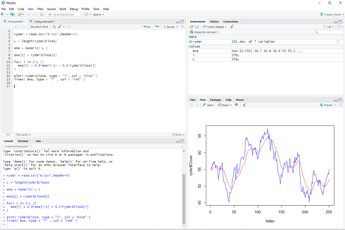
There is no "exponential moving average" procedure in the R base package, but it can be easily calculated with a for-loop.
After loading the stock data file
ryder = read.csv("R.csv",header=T)
L = length(ryder$Close)
we create the vector ema
ema = numeric( L )
We set the first element of ema to the first close price
ema[1] = ryder$Close[1]
and then we calculate
ema[2] = 0.9*ema[1] + 0.1*ryder$[2]
ema[3] = 0.9*ema[2] + 0.1*ryder$[3]
.
.
.
in a loop:
for( i in 2:L ){
ema[i] = 0.9*ema[i-1] + 0.1*ryder$Close[i]
}
Finally, we display the prices and ema
plot( ryder$Close, type = "l", col = "blue" )
lines( ema, type = "l" , col = "red" )
At this point most tutorials would emphasize that R is an interpreted language and for-loops should be avoided at all costs.
Indeed one should use vector operations whenever possible instead of the element-by-element processing in a for loop.
However, microprocessors are so fast nowadays, that for-loops are problematic only for really large data sets imho.
exercise: Repeat the calculation, but with the volume instead of the price.
It is not clear if this actually improves the performance of a a stock portfolio, but perhaps investors sleep better using this approach ...
There is no "exponential moving average" procedure in the R base package, but it can be easily calculated with a for-loop.
After loading the stock data file
ryder = read.csv("R.csv",header=T)
L = length(ryder$Close)
we create the vector ema
ema = numeric( L )
We set the first element of ema to the first close price
ema[1] = ryder$Close[1]
and then we calculate
ema[2] = 0.9*ema[1] + 0.1*ryder$[2]
ema[3] = 0.9*ema[2] + 0.1*ryder$[3]
.
.
.
in a loop:
for( i in 2:L ){
ema[i] = 0.9*ema[i-1] + 0.1*ryder$Close[i]
}
Finally, we display the prices and ema
plot( ryder$Close, type = "l", col = "blue" )
lines( ema, type = "l" , col = "red" )
At this point most tutorials would emphasize that R is an interpreted language and for-loops should be avoided at all costs.
Indeed one should use vector operations whenever possible instead of the element-by-element processing in a for loop.
However, microprocessors are so fast nowadays, that for-loops are problematic only for really large data sets imho.
exercise: Repeat the calculation, but with the volume instead of the price.
My introduction to R - step 5
An important feature of R is that one calculates with vectors and therefore can process large quantities of data in a single line.
Let's take the data from previous steps
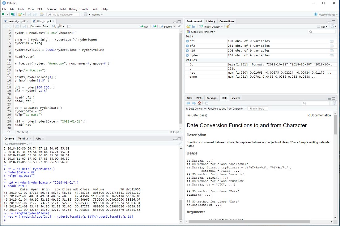
ryder = read.csv("R.csv",header=T)
and calculate the "trading range", normalized by the open, for every day
tRng = ( ryder$High - ryder$Low )/ ryder$Open
This generates the vector tRng , calculates the difference of high and low for every day, divided by the open and assigns the result to the elements of tRng, i.e. 251 * 2 calculations, all in one line.
We can now add this vector to the data frame ryder
ryder$TR = tRng
Now let's calculate the dollar trading volume in thousands for each day and add it as a column
ryder$dVol1000 = 0.001*ryder$Close * ryder$Volume
We can take a look at the first entries of the data frame with the head() procedure
head(ryder)
but we would see the same thing in window 3 top right.
If we want to store the expanded data frame in a file, we could do it as follows
write.csv( ryder, "Rnew.csv", row.names=F, quote=F )
I set the parameters so that it has the exact same format as R.csv.
You can get help with
help("write.csv")
The columns of ryder are: Date, Open, High, Low, Close, Adj.Close, Volume, ...
and we can access each column by its name
print( ryder$Close[3] )
But we can also access the elements of a data frame directly
print( ryder[3,5] )
The first index is the row and the second the column (Close is the 5-th column of ryder).
We can also slice data frames
df1 = ryder[100:200, ]
head( df1 )
Notice that the blank entry, instead of an index, means all columns.
df2 = ryder[ , 1:5]
head( df2 )
The blank entry, instead of an index, means all rows.
Until now, I have not mentioned the column Date and for a good reason - it is a bit of a mess.
The read.csv procedure interprets it as a Factor and not a date, although the entries are formatted so that R can interpret it as date.
But we can fix that
Dt = as.Date( ryder$Date )
ryder$Date = Dt
help("as.Date")
The as. family of conversion functions is quite useful in R.
This allows us to slice the data frame ryder in yet another way ...
r19 = ryder[ryder$Date > "2019-01-01",]
head( r19 )
... and concludes this step of my introduction.
exercise: Calculate the returns of ryder for each day, beginning with the 2nd day.
The return on the 2nd day is ( ryder$Close[2] - ryder$Close[1] )/ryder$Close[1] ,
the return on the 3rd day is ( ryder$Close[3] - ryder$Close[2] )/ryder$Close[2] ,
etc. Now calculate it in one line and assign the results to a vector Ret.
hint: Use L = length(ryder$Close) in your calculation ...
Let's take the data from previous steps
ryder = read.csv("R.csv",header=T)
and calculate the "trading range", normalized by the open, for every day
tRng = ( ryder$High - ryder$Low )/ ryder$Open
This generates the vector tRng , calculates the difference of high and low for every day, divided by the open and assigns the result to the elements of tRng, i.e. 251 * 2 calculations, all in one line.
We can now add this vector to the data frame ryder
ryder$TR = tRng
Now let's calculate the dollar trading volume in thousands for each day and add it as a column
ryder$dVol1000 = 0.001*ryder$Close * ryder$Volume
We can take a look at the first entries of the data frame with the head() procedure
head(ryder)
but we would see the same thing in window 3 top right.
If we want to store the expanded data frame in a file, we could do it as follows
write.csv( ryder, "Rnew.csv", row.names=F, quote=F )
I set the parameters so that it has the exact same format as R.csv.
You can get help with
help("write.csv")
The columns of ryder are: Date, Open, High, Low, Close, Adj.Close, Volume, ...
and we can access each column by its name
print( ryder$Close[3] )
But we can also access the elements of a data frame directly
print( ryder[3,5] )
The first index is the row and the second the column (Close is the 5-th column of ryder).
We can also slice data frames
df1 = ryder[100:200, ]
head( df1 )
Notice that the blank entry, instead of an index, means all columns.
df2 = ryder[ , 1:5]
head( df2 )
The blank entry, instead of an index, means all rows.
Until now, I have not mentioned the column Date and for a good reason - it is a bit of a mess.
The read.csv procedure interprets it as a Factor and not a date, although the entries are formatted so that R can interpret it as date.
But we can fix that
Dt = as.Date( ryder$Date )
ryder$Date = Dt
help("as.Date")
The as. family of conversion functions is quite useful in R.
This allows us to slice the data frame ryder in yet another way ...
r19 = ryder[ryder$Date > "2019-01-01",]
head( r19 )
... and concludes this step of my introduction.
exercise: Calculate the returns of ryder for each day, beginning with the 2nd day.
The return on the 2nd day is ( ryder$Close[2] - ryder$Close[1] )/ryder$Close[1] ,
the return on the 3rd day is ( ryder$Close[3] - ryder$Close[2] )/ryder$Close[2] ,
etc. Now calculate it in one line and assign the results to a vector Ret.
hint: Use L = length(ryder$Close) in your calculation ...
Subscribe to:
Comments (Atom)