My introduction to R - step 4

Linear regression is the oldest machine learning method. It is widely used and allows one to extrapolate from the known to the unknown.
Large fortunes have been made and lost with the help of linear regression models ...
In the following we will calculate a linear model on a sample of stock prices and then compare it against stock prices "out of sample".

If you start RStudio, it might show an R script with leftovers from the previous exercise - I suggest you create a new script (menu bar: File > New File > R Script).

We read the R.csv file from step 2 with read.csv:
ryder = read.csv("R.csv",header=T)
and then store the length of the vector ryder$Close:
L = length(ryder$Close).

We calculate two variables we will later use for displays:
maxP = max(ryder$Close) + 5.0
minP = min(ryder$Close) - 5.0

The file should contain more than 250 data points (one year of stock prices) and we use the first 200 days for in sample estimation.
days = 1:200
prc = ryder$Close[days]

Notice that ryder$Close is a vector and ryder$Close[1] is the first element we want and ryder$Close[200] the last of the in-sample period. ryder$Close[days] is equivalent to ryder$Close[1:200] and therefore prc is a vector which stores the first 200 elements of ryder$Close.
This slicing of vectors is quite often used and would work even if the elements of days would not be sequentially ordered.

Now we can plot the prices as a function of each day:
plot( days, prc, ylim = c(minP,maxP) )

We calculate the linear regression model with the lm() procedure:
mdl = lm( prc ~ days)
Notice the ~ used in the procedure call (which may or may not not be easy to find on a non-US keyboard).
We can print a summary of the linear model with
summary(mdl)
and we get the two coefficients (intercept and slope) using coef(mdl), which returns a vector.
Therefore we can calculate the linear model as
lin = coef(mdl)[1] + coef(mdl)[2]*days

and add the line to our plot with the lines() procedure:
lines( days, lin, type="l", col="red")



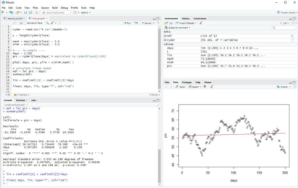
You can either execute your script step by step with Ctrl-Enter or type the script first and then execute the whole thing by selecting from the menu: Code > Run Region > Run All

Now we look at the out-of-sample data:
days = 201:L
prc = ryder$Close[days]
and display it with
plot( days, prc, ylim = c(minP,maxP) )

We calculate the out-of-sample model
lin = coef(mdl)[1] + coef(mdl)[2]*days
and add the line to the plot
lines( days, lin, type="l", col="red")



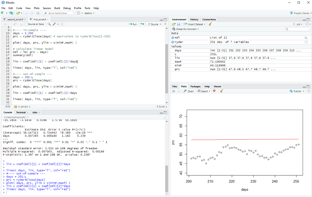
We could now calculate the out-of-sample error (it is quite obvious that the error exceeds the variance of the data in this example 8-) and perhaps repeat the procedure for many different stocks and time periods to check if the linear model has any useful predictive value.
However, this concludes step 4 of my introduction

exercise: Repeat this regression exercise, but use the Volume instead of the Close ...

My introduction to R - step 3

In the previous two steps we encountered variables and constants of different types.
Let's take a closer look ...

In R one creates variables by giving them a name and assigning a value, as we did with
the_answer = 6*7

The name can consist of letters, numbers and the two characters _ and .
but do not use _ or . or a number as the first character.
Examples of valid names:
var1
the_strength_of_Luisa
dog.leg

There are reserved words, which cannot be used to name variables, you can get a list with the help procedure:
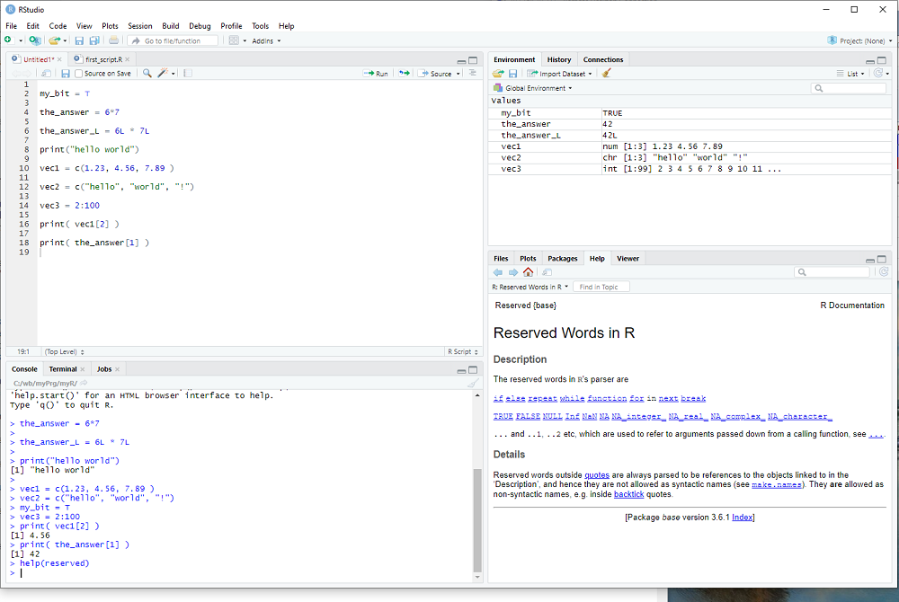
help(reserved)
You probably don't want this line in your R script, so I suggest you type help(reserved) in window 2 bottom left and hit Enter. Indeed window 2 is a fully functional R terminal and I use it to try out things and keep whatever code I want saved in window 1, i.e. in my R script.

Whenever we create a variable, R figures out the data type from the assigned value and/or operation(s).
We already encountered several different data types:

logical: TRUE or FALSE , abbreviated as T or F (e.g. the parameter header=T in the read.csv procedure)

numeric: the_answer = 6*7 was our first example, 3.1415 would be another

integer: R does not distinguish 6 from 6.0 , but if one wants to explicitly use a whole number
it needs do be indicated with the letter L, e.g. 6L
the_answer = 6L*7L
is now an integer and not a numeric variable.

strings: We have used the string "blue" in the plot procedure and one can display strings e.g. with the print procedure
print("blue")


R uses vectors as basic building blocks, collections of elements with the same data type.
ryder$Close was an example of a vector.
But the_answer was a vector too, just a small vector with 1 element only.
We access the elements of a vector with the [] operator, so that
ryder$Close[3]
would be the 3rd element of the vector, i.e. the 3rd entry of the data column.
And the_answer[1] would be the one and only element of the vector the_answer.
Notice that vector indices begin with 1 and not 0 as in some other programming languages.

One can generate a vector e.g. with the function c(), used so often that it has a really short name:
vec1 = c(1.1, 2.7, 3.2, 4.6)
creates a numeric vector with 4 elements.
vec2 = c("me","my","friend","and","you")
creates a vector with 5 strings as elements.

Last but not least, the : operator can be used to create a specific vector of integers
vec3 = 2:7
creates a vector with 5 integers as elements, the whole numbers 2, 3, 4, 5, 6, 7.



exercise: Create vectors of different sizes and types - watch in window 3 what it displays for each one.