My introduction to R - step 4

Linear regression is the oldest machine learning method. It is widely used and allows one to extrapolate from the known to the unknown.
Large fortunes have been made and lost with the help of linear regression models ...
In the following we will calculate a linear model on a sample of stock prices and then compare it against stock prices "out of sample".

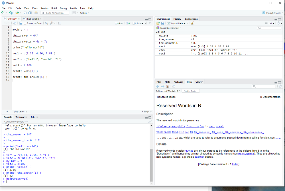
If you start RStudio, it might show an R script with leftovers from the previous exercise - I suggest you create a new script (menu bar: File > New File > R Script).

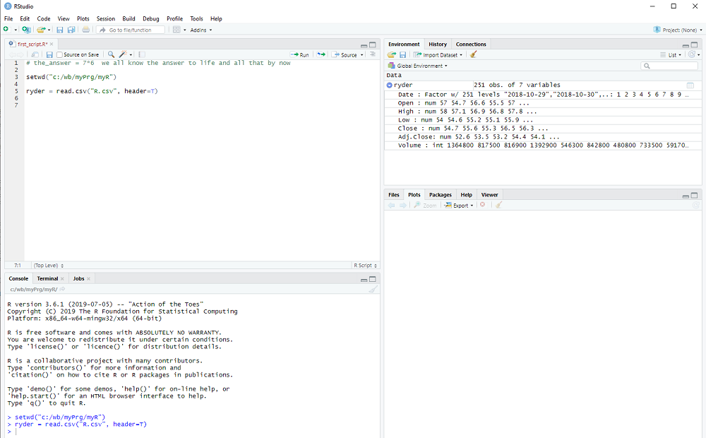
We read the R.csv file from step 2 with read.csv:
ryder = read.csv("R.csv",header=T)
and then store the length of the vector ryder$Close:
L = length(ryder$Close).

We calculate two variables we will later use for displays:
maxP = max(ryder$Close) + 5.0
minP = min(ryder$Close) - 5.0

The file should contain more than 250 data points (one year of stock prices) and we use the first 200 days for in sample estimation.
days = 1:200
prc = ryder$Close[days]

Notice that ryder$Close is a vector and ryder$Close[1] is the first element we want and ryder$Close[200] the last of the in-sample period. ryder$Close[days] is equivalent to ryder$Close[1:200] and therefore prc is a vector which stores the first 200 elements of ryder$Close.
This slicing of vectors is quite often used and would work even if the elements of days would not be sequentially ordered.

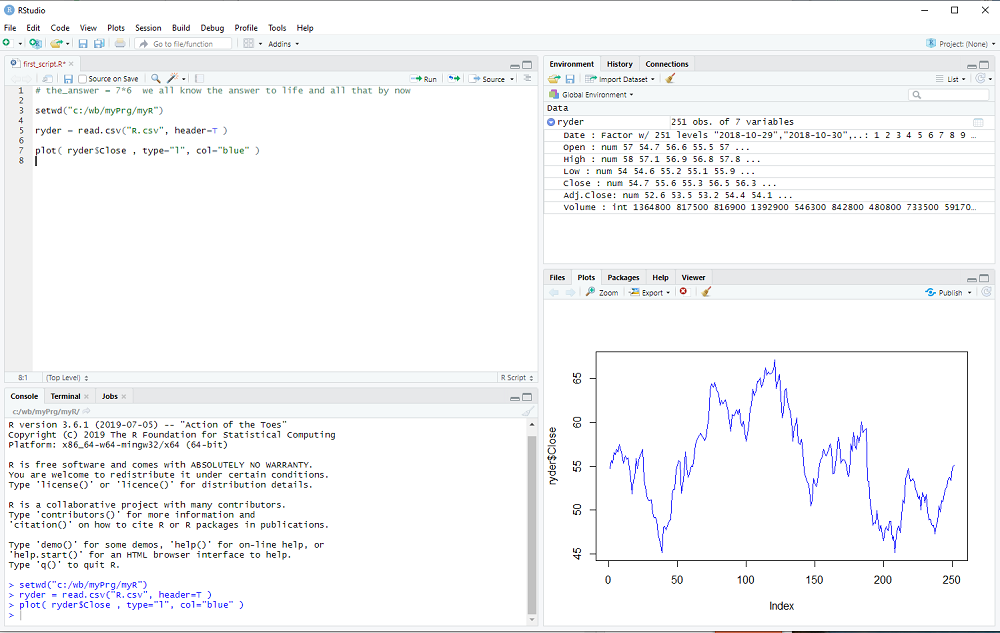
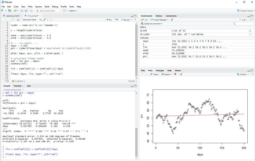
Now we can plot the prices as a function of each day:
plot( days, prc, ylim = c(minP,maxP) )

We calculate the linear regression model with the lm() procedure:
mdl = lm( prc ~ days)
Notice the ~ used in the procedure call (which may or may not not be easy to find on a non-US keyboard).
We can print a summary of the linear model with
summary(mdl)
and we get the two coefficients (intercept and slope) using coef(mdl), which returns a vector.
Therefore we can calculate the linear model as
lin = coef(mdl)[1] + coef(mdl)[2]*days

and add the line to our plot with the lines() procedure:
lines( days, lin, type="l", col="red")



You can either execute your script step by step with Ctrl-Enter or type the script first and then execute the whole thing by selecting from the menu: Code > Run Region > Run All

Now we look at the out-of-sample data:
days = 201:L
prc = ryder$Close[days]
and display it with
plot( days, prc, ylim = c(minP,maxP) )

We calculate the out-of-sample model
lin = coef(mdl)[1] + coef(mdl)[2]*days
and add the line to the plot
lines( days, lin, type="l", col="red")



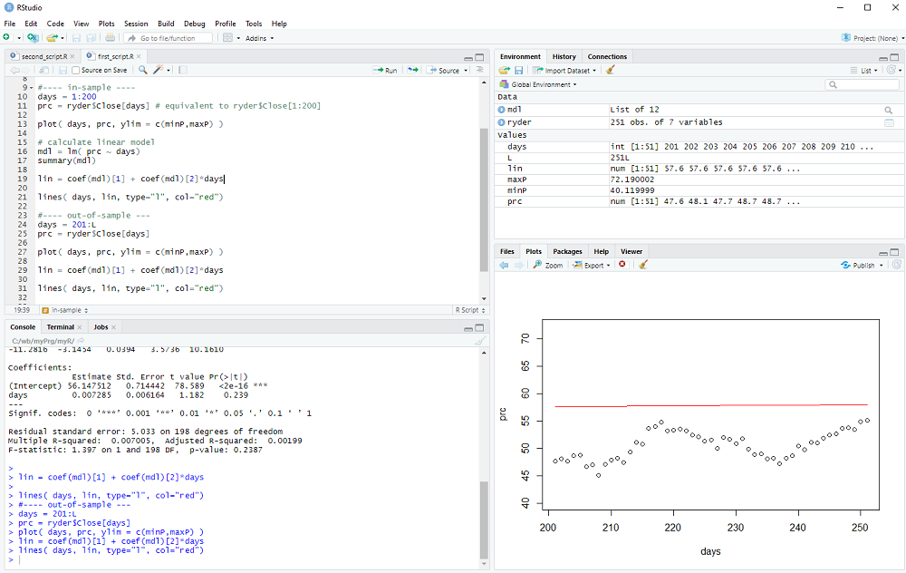
We could now calculate the out-of-sample error (it is quite obvious that the error exceeds the variance of the data in this example 8-) and perhaps repeat the procedure for many different stocks and time periods to check if the linear model has any useful predictive value.
However, this concludes step 4 of my introduction

exercise: Repeat this regression exercise, but use the Volume instead of the Close ...

My introduction to R - step 3

In the previous two steps we encountered variables and constants of different types.
Let's take a closer look ...

In R one creates variables by giving them a name and assigning a value, as we did with
the_answer = 6*7

The name can consist of letters, numbers and the two characters _ and .
but do not use _ or . or a number as the first character.
Examples of valid names:
var1
the_strength_of_Luisa
dog.leg

There are reserved words, which cannot be used to name variables, you can get a list with the help procedure:
help(reserved)
You probably don't want this line in your R script, so I suggest you type help(reserved) in window 2 bottom left and hit Enter. Indeed window 2 is a fully functional R terminal and I use it to try out things and keep whatever code I want saved in window 1, i.e. in my R script.

Whenever we create a variable, R figures out the data type from the assigned value and/or operation(s).
We already encountered several different data types:

logical: TRUE or FALSE , abbreviated as T or F (e.g. the parameter header=T in the read.csv procedure)

numeric: the_answer = 6*7 was our first example, 3.1415 would be another

integer: R does not distinguish 6 from 6.0 , but if one wants to explicitly use a whole number
it needs do be indicated with the letter L, e.g. 6L
the_answer = 6L*7L
is now an integer and not a numeric variable.

strings: We have used the string "blue" in the plot procedure and one can display strings e.g. with the print procedure
print("blue")


R uses vectors as basic building blocks, collections of elements with the same data type.
ryder$Close was an example of a vector.
But the_answer was a vector too, just a small vector with 1 element only.
We access the elements of a vector with the [] operator, so that
ryder$Close[3]
would be the 3rd element of the vector, i.e. the 3rd entry of the data column.
And the_answer[1] would be the one and only element of the vector the_answer.
Notice that vector indices begin with 1 and not 0 as in some other programming languages.

One can generate a vector e.g. with the function c(), used so often that it has a really short name:
vec1 = c(1.1, 2.7, 3.2, 4.6)
creates a numeric vector with 4 elements.
vec2 = c("me","my","friend","and","you")
creates a vector with 5 strings as elements.

Last but not least, the : operator can be used to create a specific vector of integers
vec3 = 2:7
creates a vector with 5 integers as elements, the whole numbers 2, 3, 4, 5, 6, 7.



exercise: Create vectors of different sizes and types - watch in window 3 what it displays for each one.

My introduction to R - step 2

R is mainly used for statistics, machine learning etc. and to do that we need interesting data.
One place which generates a lot of data is the US stock market and therefore we head over to
finance.yahoo.com
to grab some interesting free samples.
On the right hand side there is a box Quote Lookup and we enter R as the ticker symbol, which gives us price and other information for Ryder System Inc. - a company which has little to do with the R programming language.
We click on historical data, select a time period (1 year is fine), push the "Apply" button and then click on "Download Data".
Save the file R.csv to the myR folder (or wherever you like to store it).

Now it is time to start RStudio and it will probably open with the one-line script we made in the previous step.
However, we already know the_answer and we "comment out the line" by putting a # character in front of it.
R ignores comments and RStudio colors them green, they are only there for us human beings to better understand what we did and want to do ...

Before we take a look at the R.csv file, we set the "working directory" in RStudio: In the menu click on Tools and select Tools > Global Options ... and then select General (which should be the default selection anyways). Go to "Default working directory ..." and select the path to your myR folder (or wherever you stored the R.csv file) by pushing the Browse button; then hit apply and eventually this will need a restart of RStudio to take effect.
Alternatively, one can call the R procedure setwd in the R script to set that path:
setwd("c:/path/to/my/folder/myR")
Notice that R uses forward slashes, even on windows, betraying its unix heritage.

Now we are ready to load the stock data of Ryder System Inc. using the read.csv procedure:
ryder = read.csv( "R.csv", header=T )

After we execute the line with Ctrl-Enter, window 3 top right will display the variable ryder and by clicking on the arrow next to it we see more of what it contains.
This is how RStudion looks at this point:



The columns that we saw on the Yahoo webpage are all there: Date, Open, High, ...
R tells us what type they are, num for decimal number, int for integers, etc. and shows us some examples.
In other words, read.csv converts the comma separated values (aha, this is what csv stands for) of the file into a collection of variables, which is called dataframe in R.

We can access each column in the dataframe using its name and the $ operator, e.g. ryder$Close
This works, because we used header=T in the read.csv procedure (T stands for TRUE).

If the data comes in a different file format, e.g. variables separated by tabs is popular, the read.table procedure might be used to import data into R.

We will now take a first look at the data using the plot procedure:
plot( ryder$Close, type="l", col="blue" )

You may notice that a window popped up, listing the available columns in ryder while you typed. You can use that window to select Close without further typing.
RStudio now looks like this:



This concludes the 2nd step of my introduction. Don't forget to save your R script with File > Save in the menubar.

exercise: Click on the line with the plot procedure and then hit F1. The help text for the plot procedure should appear in window 4, bottom right.
Try different types and colors with your plot ...

My introduction to R - step 1

You want to know how to actually do machine learning, or you want to know how those finance quants do their job, or you just want to add a valuable skill to your cv ...
In other words, you want to learn R (btw what programming language do pirates use? Rrrrrrr ).
But you want to learn in small steps, easy to follow along and yet with visible results already after a few steps. Well, you have come to the right place and as additional benefit you can post questions and comments whenever you want or need to know more ...

Just one important disclaimer: I am just another user, perhaps with a bit more experience than you at the moment; but I still peek into my R for Dummies book every now and then.
I am certainly not an R guru.

The first thing we need to do is install R and Rstudio.

Install R: Go to www.r_project.org, click on download R and select a mirror.
If you live e.g. in the UK, you might select the one from Imperial College of London.
There you select your operating system and click on install R for the first time (if you are on Windows) or save the R-3.61.pkg package (if you are on a Mac), or whatever is the latest package. Linux users need to select their distribution etc.

Install RStudio: Go to rstudio.com and click on the download rstudio button. Choose the free version of RStudio Desktop and select the installer for your operating system or Linux distribution etc. ...

If you have problems with the installation, please post a comment or ask Google for help.

But if all goes well, you should be able to start RStudio and it will look like this:



Click on File in the menu bar and select File > New File > R script.
RStudio will now look like this:



It contains 4 sub-windows and I have scribbled numbers into the screenshot to better explain what they are.
1> top left: This window displays our R script and we will edit it there.
2> bottom left: This window shows executed commands, error messages, etc.
3> top right: This window shows all the different data and variables we will generate.
4> bottom right: This window is used for various displays, help text etc.

In order to get really started, we type our first R script in sub-window 1 and it contains only one line:
the_answer = 7*6
After typing that, with the cursor still on the line, press Ctrl-Enter to "execute" it.
Alternatively, we could have selected Code from the menu bar and then "Run Selected Line(s)".
The RStudio screen should now look like this:



In the top left window 1 we still see our R script, containing one line.
In the bottom left window 2 we see that R executed our line without error and
in the top right window 3 we see that R created a variable named the_answer with the value 42.
R actually did three things: It created the_answer, executed the arithmetic operation 7*6 and then assigned the outcome of that operation to the_answer.

I read that some people have a problem with the = operator when learning to program in some cases. R has a solution for that, one can also use the assignment operator <- instead of the equal sign. So we could have written
the_answer <- 7*6
with the exact same outcome. In older texts this assignment operator is often used instead of = and you should know that it really makes no difference.

Now we want to save our script and I recommend that you create a folder somewhere on your pc, which you will use to store the R scripts and data files we use in this tutorial; I named my folder myR and will reference it in future steps with this name.
Once you have created and/or selected a place on your pc, select File on the menu bar, click on Save As..., navigate to myR and choose a name for your script, e.g. first_step.R
I recommend that your script files end with .R

This concludes the first step of my introduction.

exercise: Click on Help in the menu bar, select R Help and browse e.g. "An Introduction to R", in window 4.

Just one more thing. At the end of your RStudio exercise, select File from the menu and click on Quit Session...; if you are prompted to save the workspace image select No, which means that the next time you start RStudio, you start from a clean slate.